Table of Contents
The Main GUI Window
Basically the “control room” of the TA Toolbox and especially its GUI. From here, you can access every single function of the toolbox, and what is even more, completely GUI-based.
Introduction
How to use the GUI? A very brief introduction.
If in a hurry
![]() Given the complexity of the main GUI window, it is not easy to give you a one-minute introduction. But the good news is: The GUI tries to be easy-to-use by design. Most of the things should be self-explaining. Nevertheless, following a very quick rush through the different panels and their main functions.
Given the complexity of the main GUI window, it is not easy to give you a one-minute introduction. But the good news is: The GUI tries to be easy-to-use by design. Most of the things should be self-explaining. Nevertheless, following a very quick rush through the different panels and their main functions.
1. Load data
The first step is to load one or more datasets. That can be done via the “load” panel that is accessed by pressing the <key>Load</key> button.
2. Toggle visibility
After loading one or more datasets from files, you need to make the data appear on the main axis to the left. Therefore, hit the <key>Datasets</key> button that will give you all necessary control.
3. Sliders
You can scroll through a 2D dataset in both directions, you can scale the data in both dimensions and you can displace the data in two dimensions. Therefore, press the <key>Slider</key> button that provides you with a convenient display of the current slider values in both data points and actual units of the axes.
4. Measure
One of the most natural things to do with a 2D or 1D dataset displayed is to measure distances between different points. This can be done with the “Measure” panel that will appear once you press the <key>Measure</key> button.
5. Display
Once you succeeded in displaying the data in a meaningful way, you may want to either export the currently displayed data to a file (MATLAB fig, EPS, PDF, PNG, …) or to modify the figure as a conventional MATLAB figure.
Furthermore, if the data you loaded do not contain the necessary information for the axis labels, you may want to correct or set them as well.
Either functionality is easily accessible: Just press the <key>Display</key> button.
6. Processing
For the advanced user, the “Processing” panel will provide all sorts of functions for data manipulation, such as accumulating different data sets.
7. Analysis
To finally analyse your data, you might want to fit different functions to them, simulate data or perform deconvolutions. All those functions are grouped within and accessible from the “Analysis” panel.
8. MFE
A special feature only used for a minority of TA data is the handling of measurements of the magnetic field effect (MFE). In this case, TA time traces have been recorded both without and with a static field applied. The “MFE” panel lets you perform the usual tasks on those data.
9. Configure
Just added for completeness in this short description: The “Configure” panel lets you at least partly adjust the behaviour of the TA toolbox and especially the GUI to your needs.
To the gentle reader
The main GUI window is the “control room” of the TA Toolbox and especially its GUI. From here, you can access every single function of the toolbox.
Accessing the Main GUI
Starting the Main GUI is the only time when you might want to use the command line. Simply type:
TAgui;
and hit <key>Enter</key>. That should start the GUI and a window should appear that looks similar to the one shown below.
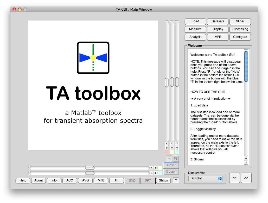
GUI layout
Basically, the main GUI window is divided into two main parts: The main axis to the left, with all its controls surrounding it, and the panels to the right. You can switch between the panels on the right with the buttons on the top or via shortcuts <key>Ctrl-1</key> to <key>Ctrl-9</key>.
Additionally, on the bottom below the main axis is a row of “function keys” that open one-by-one additional GUI windows, and that can be accessed via the shortcuts <key>F1</key> to <key>F10</key> (therefore “function” buttons).
More details to all the different panels and the meaning of their control elements can be found in the respective help topics: