Table of Contents
Main GUI: Display Panel
The display panel is currently by far the most complex single panel of the main GUI window, divided into six pages (subpanels), each dealing with a related subset of display-related settings.
Page 1: Axis labels and limits
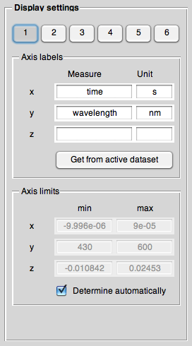
Both axis labels and axis limits can be set manually for all three axes.
The axis labels can be determined from the currently active dataset (if possible), the axis limits are normally set to “automatic”, meaning that they are optimised to fit all currently visible datasets into the axes.
Page 2: Grid, Legend, Normalize, Highlighting
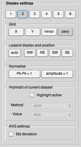
Grid
A zero line is displayed by default in case of the 1D representations (but not for the 2D display), grids in x and y direction can be added independently, and the minor grid can be added (simultaneously for both axes).
In this particular case, x and y refers to the abscissa and ordinate of the current display, not to the x, y, and z dimensions of the dataset, as everywhere else.
Legend
Legends are only displayed in 1D mode. You can determine the legend position manually (NW, NE, SW, SE) or let Matlab® determine what it thinks is the “optimal” position.
Normalise
As signal intensity of TREPR spectra depends in a far from straightforward way on a couple of both experimental (i.e., related to the current setup) and inherent (overlap and thus cancellation of absorptive and emissive lines in the spectrum) parameters, it normally cannot be used for quantitative analysis of the spectra.
Therefore, to directly compare, e.g., the decay of two different time traces, or the shape of two different spectra, normalisation of the datasets is quite helpful.
The two different types of normalisation provided with the GUI here is peak-peak and amplitude normalisation, whereas the former sets the complete peak-to-peak-amplitude to one, the latter the amplitude measured between zero and maximum.
Highlight of current dataset
To be able to distinguish between the currently active and other visible datasets, by default the currently active dataset is highlighted with blue colour, with all other datasets displayed with black lines.
Here, both method and value for the given method of highlighting can be controlled, and one can switch off the highlighting completely. The latter is of special interest for exporting figures, where no highlighting of the “currently active dataset” is necessary, and indeed rather confusing.
Page 3: Line settings
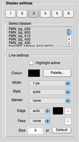
To distinguish between different (visible) datasets, the line settings of each dataset can be controlled as far as Matlab® allows to do so, meaning line colour, width, style, and marker.
Please note: If “highlight currently active” is switched on, it will most probably interfere with the settings. Therefore, if the line settings seem not to work properly, you should switch of the highlighting as a first step.
To show only the (unconnected) data points, set “Style” to none and choose from one of the “Markers”.
Page 4: Export figure & 1D datasets
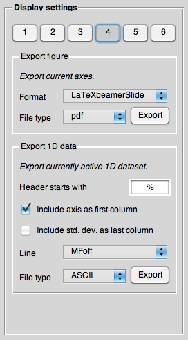
What is a GUI worth that does not allow to save the current display in an easy way to a file?
Export figure
To export the current display to a file, choose the file type (currently Matlab® FIG, EPS, PDF, PNG) and hit <key>Export</key>.
The “Format” popupmenu allows to specify a format (aspect ratio, size of the graphics) that makes it easier to use the saved figures, e.g., in reports. These formats can be fully customised using the fig2file.ini file in the same directory as the fig2file function.
Export 1D data
This function allows the user to save the currently active 1D dataset as ASCII data, mainly for further analysis and processing in other software.
Page 5: 3D display
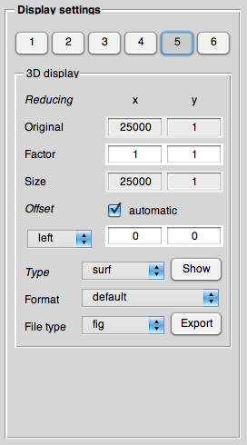
A 3D representation of 2D datasets (with intensity as third dimension) is sometimes used for an overview of a given 2D dataset. The 3D display panel allows the user to generate such datasets, that are normally restricted in their resolution (as a full 200×500 point or even larger dataset will be quite huge and slow in display).
Furthermore, these 3D views can be exported in the same way as the main display. To export the current 3D display to a file, choose the file type (currently Matlab® FIG, EPS, PDF, PNG) and hit <key>Export</key>.
Please note: If you just hit <key>Export</key> without having an actual 3D display window, no figure will be exported.
The “Format” popupmenu allows to specify a format (aspect ratio, size of the graphics) that makes it easier to use the saved figures, e.g., in reports. These formats can be fully customised using the fig2file.ini file in the same directory as the fig2file function.
Page 6: Thresholds
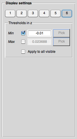
Thresholds
Allow to set a threshold in y (on a per dataset basis).