Table of Contents
MFE GUI: MFE Panel
The MFE panel lets you set all the parameters necessary for calculating the MFE and lets you perform the actual MFE calculation.
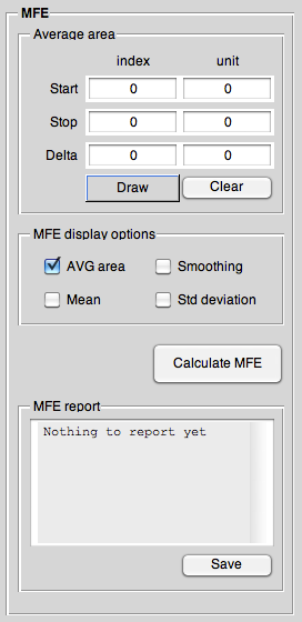
Average area
This is the area the MFE gets calculated for (as a time-averaged MFE).
The average area can be defined in terms of start and stop values or a start and a delta value.
Therefore: If you change the delta value, it will change the stop value as well, but keep the start value constant. If your delta value is too big for the current settings of the start value and given the size of the dataset in the particular dimension, then the delta value gets reset to the maximum possible value for the given start value.
MFE display options
The options here let you control what gets displayed in the main axis of the MFE GUI window.
AVG area
Display area that is averaged over for calculating the MFE. Even if you switch this off, it gets displayed in the small window on the bottom left.
Smoothing
When in “1D along y” display mode and in one of the MFE display modes that display the “DeltaMF” trace, show smoothed trace. The smoothing filter settings can be set via the “Settings” panel. Mean
Display mean value(s) of current trace(s) as horizontal line(s) if in “1D along x” display mode. This may help to visualise the mean of a given trace.
Std deviation
If in “1D along x” display mode, display standard deviation value(s) of the calculated mean value(s) of current trace(s) as horizontal line(s)
If in “1D along y” display mode, these values get displayed as error bars.
This may help to visualise the standard deviation of the calculated mean value of a given trace.
Calculate MFE button
Pressing this button will result in calculating the MFE for the given trace with the given area to average over. The results will be displayed in the report subpanel below the button. If no area was selected, this will be stated in the report subpanel instead.
To calculate the absolute MFE, normally the following formula is used:
<latex> \text{MFE} = \frac{1}{t_2-t_1}\int_{t_1}^{t_2}\frac{\Delta\Delta A(B,t)}{|\Delta A(0\;{\rm mT},t)|}{\rm d}t </latex>
Due to possible issues with very noisy datasets where taking the absolute of the MFon trace would cause problems, a slightly altered version of the above formula is used that gives as well the correct sign of the MFE:
<latex> \text{MFE} = \frac{1}{t_2-t_1}\int_{t_1}^{t_2}\frac{\Delta\Delta A(B,t)}{\Delta A(0\;{\rm mT},t)}{\rm d}t*\text{sign}\{\Delta A(0\;{\rm mT},t)\} </latex>
The MFE may also be calculated as a function of time: at any time t the instantaneous MFE can be calculated as the ratio of ΔΔA(B,t) and ΔA(0 mT,t). However, for noisy data, or at points where ΔA(0 mT,t) is close to zero, this can lead to large variations in the calculated MFE. Therefore, use of time-averaged MFEs is preferential.
MFE report
Results of the MFE calculation.
The <key>Save</key> button lets you choose a file to save the report to.