Inhaltsverzeichnis
The Fit GUI window
Fitting arbitrary functions to your data in 1D
Introduction
A rather short introduction to the Fit GUI.
If in a hurry
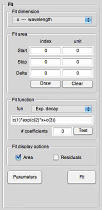
![]() You want to fit basic functions (e.g., exponential) to your data in 1D, such as determining the decay of a time trace? The Fit GUI is the place to go. Select your dataset and 1D representation (via the „Display“ panel), switch to the „Fit“ panel, set your fit area, select the function to be fitted to the data, press „Fit“, and hopefully you're done. The fitted values for the coefficients will be listed together with a full report of the fit process below the main axis.
You want to fit basic functions (e.g., exponential) to your data in 1D, such as determining the decay of a time trace? The Fit GUI is the place to go. Select your dataset and 1D representation (via the „Display“ panel), switch to the „Fit“ panel, set your fit area, select the function to be fitted to the data, press „Fit“, and hopefully you're done. The fitted values for the coefficients will be listed together with a full report of the fit process below the main axis.
To the gentle reader
The Fit GUI is dedicated to the task of 1D data fitting, meaning that it allows you to fit a set of (standard) functions to a selected 1D representation of your data. Furthermore, it gives you plenty of control over the exact fit conditions, such as the area to use for the fit, the fit functions, the behaviour of the fit method used, and the initial guesses of the coefficients used for fitting.
As fitting is rather an analysis than a data processing task, there is no means of applying whatever fit to the data and return that to the main GUI. Nevertheless, you can save the report generated by the fitting to a file, thus allowing you to save it to your other records of that particular dataset.
As data fitting is a rather complicated matter, this Fit GUI is designed with the standard cases in mind, such as fitting a decay of a time trace.
There is ideas to allow the user to fit arbitrary, user-defined 1D functions to the data. Furthermore, an additional idea would be to automatically integrate the „Matlab Optimization Toolbox“, if it is available on the system.
Accessing the Fit GUI
There are two ways how to access the Fit GUI: Either press the <key>Fit</key> button located in the row of buttons at the bottom left of the Main GUI window, or press <key>F7</key>. This will open the Fit GUI window, as shown below.
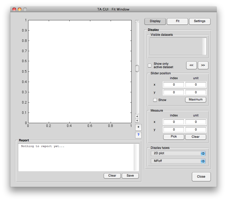
GUI layout
Basically, the Fit GUI window is divided into three panels that are all located to the right. You can switch between them with the buttons on the top or via shortcuts <key>Ctrl-1</key> to <key>Ctrl-3</key>.
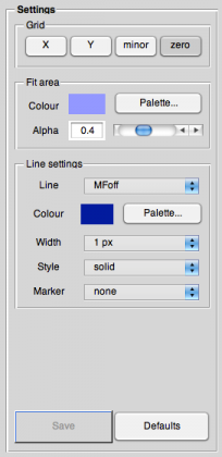
More details to all the different panels and the meaning of their control elements can be found in the respective help topic:
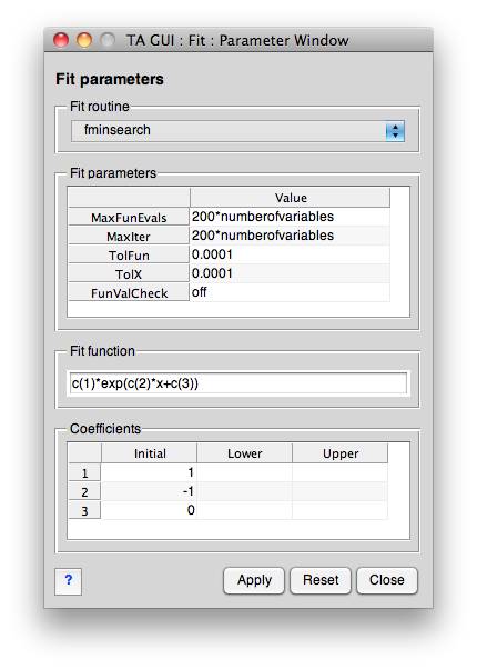
Furthermore, there are two more help topics, covering the „Parameters window“ and the contents and structure of the report that gets displayed below the main axis:
What follows is a sketch of the typical operation of this GUI.
Normal operation
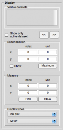
Normally, you simply go through the first two panels, „Display“ and „Fit“, first deciding about which dataset to use for fitting, and about the proper 1D representation. Then you select the area the function should be fitted to, select a function (and method) to fit to the data, probably check the initial guesses for the coefficients (via the parameters window that opens when you press the <key>Parameters</key> button), and then simply hit <key>Fit</key>.
After you did that, you will see the result in the main axis, where you can inspect it in the ususal way. All controls for this can be found in the display panel on the right.
The zoom function is started by pressing the button with the <key>+</key>, directly below the slider right to the main axis. To stop zooming, simply press the zoom button (with the <key>+</key>) again. If you want to reset the display, simply click once on the dataset in the dataset list.
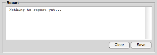
Additionally, you will find a summary of the performed action in the report panel below the main axis.